安裝

TensorFlow分為CPU和GPU兩個版本军拟，如果系統(tǒng)沒有NVIDIA? GPU炸裆，就安裝CPU版本，GPU版本的TensorFlow計(jì)算速度更快迁霎，如果滿足以下要求，可以安裝GPU版本

• CUDA? Toolkit 8.0. CUDA是一種由NVIDIA推出的通用并行計(jì)算架構(gòu)百宇，該架構(gòu)使GPU能夠解決復(fù)雜的計(jì)算問題考廉。它包含了CUDA指令集架構(gòu)（ISA）以及GPU內(nèi)部的并行計(jì)算引擎。CUDA? Toolkit是一種針對支持CUDA功能的GPU（圖形處理器）的C語言開發(fā)環(huán)境携御。
• CUDA? Toolkit 8.0的NVIDIA驅(qū)動
• cuDNN v5.1.是用于深度神經(jīng)網(wǎng)絡(luò)的GPU加速庫
• 顯卡的CUDA計(jì)算能力在3.0以上

安裝方式

• pip
  原生pip直接安裝TensorFlow而不需要通過虛擬環(huán)境昌粤，因此pip安裝的TensorFlow存放于其他python庫的路徑，并且啄刹，可以在計(jì)算機(jī)的任何路徑下運(yùn)行TensorFlow
  python3.5版本里涮坐，安裝CPU版本在命令提示符中鍵入pip install --upgrade tensorflow，安裝GPU版本鍵入pip install --upgrade tensorflow-gpu
  截止17年5月TensorFlow還不支持在python3.6中pip安裝
• Anaconda
  可以用conda指令創(chuàng)建虛擬環(huán)境誓军，但是推薦使用在anaconda下pip install.創(chuàng)建TensorFlow環(huán)境安裝袱讹，TensorFlow庫存在于創(chuàng)建的虛擬環(huán)境中，運(yùn)行時有所限制昵时。

TensorFlow起步

起步前的準(zhǔn)備工作：python的編程基礎(chǔ)捷雕、矩陣的簡單數(shù)學(xué)知識、機(jī)器學(xué)習(xí)

TensorFlow提供多種API壹甥。底層API(TensorFlow Core)提供完整的程序控制救巷。高級API建立在core之上，高級API更加容易學(xué)習(xí)應(yīng)用盹廷。像tf.contrib.learn幫助你管理數(shù)據(jù)集征绸，學(xué)習(xí)器，訓(xùn)練和推斷俄占。注意名字中包含contrib的高級API還在開發(fā)當(dāng)中管怠，在以后的版本可能會改變或者廢棄。

指南先介紹底層API缸榄，之后會用tf.contrib.learn來得到相同的模型渤弛。了解core可以更加了解在高級API使用中的內(nèi)部運(yùn)行機(jī)制。

Tensors

TensorFlow的數(shù)據(jù)核心單元是tensor(張量)甚带∷希可以把張量想象成一個n維的數(shù)組或列表。張量的rank(秩)就是維度的數(shù)量

3 # a rank 0 tensor; this is a scalar with shape []
[1. ,2., 3.] # a rank 1 tensor; this is a vector with shape [3]
[[1., 2., 3.], [4., 5., 6.]] # a rank 2 tensor; a matrix with shape [2, 3]
[[[1., 2., 3.]], [[7., 8., 9.]]] # a rank 3 tensor with shape [2, 1, 3]

TensorFlow Core

導(dǎo)入TensorFlow的所有類鹰贵、方法和屬性：import tensorflow as tf

the computational graph(計(jì)算圖)

你可以認(rèn)為TensorFlow核心代碼有兩部分組成：

1. 構(gòu)建計(jì)算圖
2. 執(zhí)行計(jì)算圖
   計(jì)算圖是由TensorFlow operation(節(jié)點(diǎn))組成晴氨。讓我們構(gòu)建一個簡單的計(jì)算圖。每個節(jié)點(diǎn)有0或更多張量作為輸入然后產(chǎn)生一個張量作為輸出碉输。有一類節(jié)點(diǎn)是常量籽前。所有的TensorFlow常量沒有輸入，它輸出一個值在內(nèi)部存儲。我們創(chuàng)建兩個浮點(diǎn)型常量node1和node2如下：

node1 = tf.constant(3.0, tf.float32)
node2 = tf.constant(4.0) # also tf.float32 implicitly
print(node1, node2)

打印結(jié)果

Tensor("Const:0", shape=(), dtype=float32) Tensor("Const_1:0", shape=(), dtype=float32)

注意：打印node并沒有輸出3.0和4.0枝哄，而是node的本身屬性肄梨，在被計(jì)算的時候才會產(chǎn)生3.0和4.0，為了正確計(jì)算節(jié)點(diǎn)挠锥，我們必須在對話(session)中執(zhí)行計(jì)算圖众羡。session壓縮了控制和TensorFlow的狀態(tài)。

接下來的代碼構(gòu)造了session對象并用它的方法run執(zhí)行足夠的計(jì)算圖來計(jì)算node1和node2：

sess = tf.Session()
print(sess.run([node1, node2]))

于是我們可以看到期望的輸出
[3.0, 4.0]
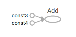
我們可以組合張量節(jié)點(diǎn)來構(gòu)造更復(fù)雜的計(jì)算蓖租，比如粱侣，我們可以使兩個常量節(jié)點(diǎn)相加來產(chǎn)生新的圖形：

node3 = tf.add(node1, node2)
print("node3: ", node3)
print("sess.run(node3): ",sess.run(node3))

最后打印出：

node3:  Tensor("Add_2:0", shape=(), dtype=float32)
sess.run(node3):  7.0

TensorFlow提供TensorBoard使計(jì)算圖可視化。

TensorBoard可視化的效果

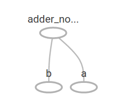
這個圖形并不完美因?yàn)樗偸钱a(chǎn)生常量結(jié)果菜秦。計(jì)算圖應(yīng)該接受外部輸入變得參數(shù)化甜害。placeholders(占位符)可以在之后提供值。

a = tf.placeholder(tf.float32)
b = tf.placeholder(tf.float32)
adder_node = a + b  # + provides a shortcut for tf.add(a, b)

上面三行代碼有點(diǎn)像我們定義兩個輸入?yún)?shù)和關(guān)于這兩個參數(shù)的節(jié)點(diǎn)的函數(shù)或匿名函數(shù)球昨。我們可以用feed_dict參數(shù)來指定提供具體值的張量給這些placeholders來計(jì)算多輸入的計(jì)算圖尔店。

print(sess.run(adder_node, {a: 3, b:4.5}))
print(sess.run(adder_node, {a: [1,3], b: [2, 4]}))

得到結(jié)果

7.5
[ 3.  7.]

在TensorBoard中的圖形顯示

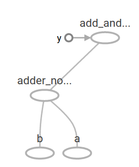
我們可以通過增加另一個節(jié)點(diǎn)使計(jì)算圖更加復(fù)雜

add_and_triple = adder_node * 3.
print(sess.run(add_and_triple, {a: 3, b:4.5}))

產(chǎn)生輸出22.5

在TensorBoard中的圖形顯示

在機(jī)器學(xué)習(xí)中，我們通常需要任意輸入主慰，為了使模型可訓(xùn)練嚣州，我們需要修改模型使在相同輸入下得到新的輸出。Variables(變量)允許我們在計(jì)算圖中增加訓(xùn)練的參數(shù)共螺「秒龋可由類型和初始值構(gòu)造：

W = tf.Variable([.3], tf.float32)
b = tf.Variable([-.3], tf.float32)
x = tf.placeholder(tf.float32)
linear_model = W * x + b

當(dāng)你調(diào)用tf.constant時，常量已經(jīng)初始化了藐不，他們的值不會再改變匀哄，相反，當(dāng)你調(diào)用tf.Variable時雏蛮，變量并沒有初始化涎嚼，為了在TensorFlow代碼中初始化所有變量，你必須調(diào)用一個特別的節(jié)點(diǎn)

init = tf.global_variables_initializer()
sess.run(init)

實(shí)現(xiàn)init是TensorFlow子計(jì)算圖初始所有全局變量的關(guān)鍵挑秉。在我們調(diào)用sess.run之前法梯，變量是為初始化的。

區(qū)別：

tf.Variable:訓(xùn)練模型時用于更新存儲參數(shù)犀概，聲明時必須提供初始值

tf.placeholder:用于得到傳遞進(jìn)來的真實(shí)的訓(xùn)練樣本立哑，不必指定初始值，可在運(yùn)行時姻灶，通過Session.run的函數(shù)的feed_dict參數(shù)指定

既然x是placeholder铛绰，我們可以訓(xùn)練linear_model來同時計(jì)算x的幾個值

print(sess.run(linear_model, {x:[1,2,3,4]}))

得到輸出
[ 0. 0.30000001 0.60000002 0.90000004]
我們構(gòu)造了一個模型但并不知道他的性能。為了在訓(xùn)練集上評估模型产喉，我們需要一個y placeholder來提供期望值至耻，和一個loss funciton(代價(jià)函數(shù))

代價(jià)函數(shù)表征了當(dāng)前模型與提供數(shù)據(jù)的距離若皱。我們將在線性回歸上用一個標(biāo)準(zhǔn)的代價(jià)函數(shù)镊叁，即當(dāng)前模型與提供數(shù)據(jù)的delta的平方和尘颓。linear_model-y構(gòu)造了一個向量，它的每個元素即使樣本的誤差delta晦譬。然后調(diào)用tf.square來平方誤差疤苹，然后調(diào)用tf.reduce_sum使所有平方誤差相加來構(gòu)造一個標(biāo)量來抽象所有樣本的誤差。

y = tf.placeholder(tf.float32)
squared_deltas = tf.square(linear_model - y)
loss = tf.reduce_sum(squared_deltas)
print(sess.run(loss, {x:[1,2,3,4], y:[0,-1,-2,-3]}))

產(chǎn)生代價(jià)值23.66

我們可以給w敛腌、b重新分配值-1卧土，1來提升性能，變量通過tf.Variable來對值初始化像樊，通過tf.assign來改變節(jié)點(diǎn)尤莺。比如，w=-1,b=1使我們的優(yōu)化參數(shù)生棍。

fixW = tf.assign(W, [-1.])
fixb = tf.assign(b, [1.])
sess.run([fixW, fixb])
print(sess.run(loss, {x:[1,2,3,4], y:[0,-1,-2,-3]}))

最終打印出代價(jià)為0

我們只是猜想得到理想的w和b的值颤霎，但機(jī)器學(xué)習(xí)的目的就是要自動找出理想的模型參數(shù)。我們將在下一節(jié)介紹

tf.train API

關(guān)于機(jī)器學(xué)習(xí)完整的討論超出了這里的范圍涂滴，無論如何友酱，TensorFlow提供了optimizers(優(yōu)化器)使每個變量朝著代價(jià)函數(shù)最小化的方向緩慢改變。最簡單的優(yōu)化器是gradient descent(梯度下降)柔纵。它使每個變量都朝代價(jià)關(guān)于變量的梯度的方向變化缔杉。通常上講，手動計(jì)算符號化的導(dǎo)數(shù)是乏味且易于出錯的搁料。TensorFlow使用函數(shù)tf.gradients可以自動產(chǎn)生導(dǎo)數(shù)或详。優(yōu)化器通常會直接完成這一步驟，比如

optimizer = tf.train.GradientDescentOptimizer(0.01)
train = optimizer.minimize(loss)

sess.run(init) # reset values to incorrect defaults.
for i in range(1000):
  sess.run(train, {x:[1,2,3,4], y:[0,-1,-2,-3]})

print(sess.run([W, b]))

打印出最終的模型參數(shù)

[array([-0.9999969], dtype=float32), array([ 0.99999082],
 dtype=float32)]

現(xiàn)在我們已經(jīng)初步實(shí)現(xiàn)了機(jī)器學(xué)習(xí)郭计，即使線性回歸并不要求太多的TensorFlow核心代碼霸琴，越復(fù)雜的模型和方法需要更多代碼。由此TensorFlow對普遍的模式拣宏、結(jié)構(gòu)沈贝、函數(shù)進(jìn)行了高級接口。我們將在下一章節(jié)學(xué)習(xí)怎樣使用這些接口勋乾。

完整代碼

完整的線性回歸模型如下：

import numpy as np
import tensorflow as tf

# Model parameters
W = tf.Variable([.3], tf.float32)
b = tf.Variable([-.3], tf.float32)
# Model input and output
x = tf.placeholder(tf.float32)
linear_model = W * x + b
y = tf.placeholder(tf.float32)
# loss
loss = tf.reduce_sum(tf.square(linear_model - y)) # sum of the squares
# optimizer
optimizer = tf.train.GradientDescentOptimizer(0.01)
train = optimizer.minimize(loss)
# training data
x_train = [1,2,3,4]
y_train = [0,-1,-2,-3]
# training loop
init = tf.global_variables_initializer()
sess = tf.Session()
sess.run(init) # reset values to wrong
for i in range(1000):
 sess.run(train, {x:x_train, y:y_train})

# evaluate training accuracy
curr_W, curr_b, curr_loss  = sess.run([W, b, loss], {x:x_train, y:y_train})
print("W: %s b: %s loss: %s"%(curr_W, curr_b, curr_loss))

最后產(chǎn)生W: [-0.9999969] b: [ 0.99999082] loss: 5.69997e-11

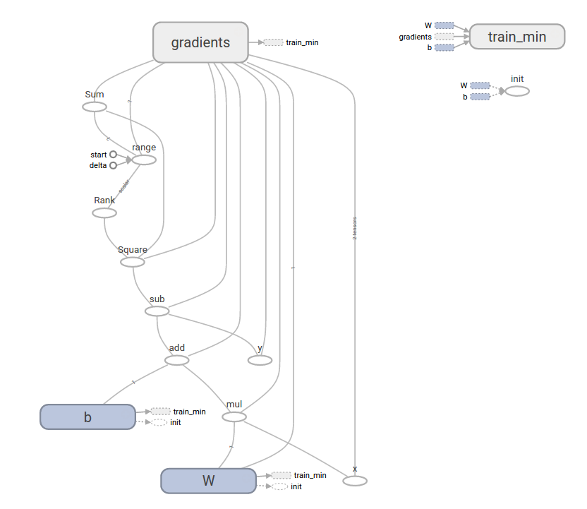
這樣復(fù)雜的代碼仍可以在tensorboard中可視化

在TensorBoard中的圖形顯示

tf.contrib.learn

tf.contrib.learn是TensorFlow中的高級庫宋下，簡化了機(jī)器學(xué)習(xí)的機(jī)制，包括：

• 運(yùn)行訓(xùn)練的循環(huán)
• 運(yùn)行測試的循環(huán)
• 管理數(shù)據(jù)集
• 管理供應(yīng)
  tf.contrib.learn包括了許多通用模型

基本用法

注意線性回歸模型用tf.contrib.learn時有多簡潔

import tensorflow as tf
# NumPy is often used to load, manipulate and preprocess data.
import numpy as np

# Declare list of features. We only have one real-valued feature. There are many
# other types of columns that are more complicated and useful.
features = [tf.contrib.layers.real_valued_column("x", dimension=1)]

# An estimator is the front end to invoke training (fitting) and evaluation
# (inference). There are many predefined types like linear regression,
# logistic regression, linear classification, logistic classification, and
# many neural network classifiers and regressors. The following code
# provides an estimator that does linear regression.
estimator = tf.contrib.learn.LinearRegressor(feature_columns=features)

# TensorFlow provides many helper methods to read and set up data sets.
# Here we use `numpy_input_fn`. We have to tell the function how many batches
# of data (num_epochs) we want and how big each batch should be.
x = np.array([1., 2., 3., 4.])
y = np.array([0., -1., -2., -3.])
input_fn = tf.contrib.learn.io.numpy_input_fn({"x":x}, y, batch_size=4,
                                              num_epochs=1000)

# We can invoke 1000 training steps by invoking the `fit` method and passing the
# training data set.
estimator.fit(input_fn=input_fn, steps=1000)

# Here we evaluate how well our model did. In a real example, we would want
# to use a separate validation and testing data set to avoid overfitting.
print(estimator.evaluate(input_fn=input_fn))

自定義模型

tf.contrib.learn沒有限制你使用它的預(yù)定義模型辑莫，假設(shè)我們想創(chuàng)建自定義的模型学歧，我們?nèi)阅軌蛟趖f.contrib.learn保持對數(shù)據(jù)集、攻擊各吨、訓(xùn)練等的高級抽象枝笨。我們將展示用底層API實(shí)現(xiàn)等價(jià)模型線性回歸。

為了定制tf.contrib.learn上的自定義模型，我們需要使用tf.contrib.learn.Estimator横浑。tf.contrib.learn.LinearRegressor也是tf.contrib.learn.Estimator的一個子類剔桨。

import numpy as np
import tensorflow as tf
# Declare list of features, we only have one real-valued feature
def model(features, labels, mode):
  # Build a linear model and predict values
  W = tf.get_variable("W", [1], dtype=tf.float64)
  b = tf.get_variable("b", [1], dtype=tf.float64)
  y = W*features['x'] + b
  # Loss sub-graph
  loss = tf.reduce_sum(tf.square(y - labels))
  # Training sub-graph
  global_step = tf.train.get_global_step()
  optimizer = tf.train.GradientDescentOptimizer(0.01)
  train = tf.group(optimizer.minimize(loss),
                   tf.assign_add(global_step, 1))
  # ModelFnOps connects subgraphs we built to the
  # appropriate functionality.
  return tf.contrib.learn.ModelFnOps(
      mode=mode, predictions=y,
      loss=loss,
      train_op=train)

estimator = tf.contrib.learn.Estimator(model_fn=model)
# define our data set
x = np.array([1., 2., 3., 4.])
y = np.array([0., -1., -2., -3.])
input_fn = tf.contrib.learn.io.numpy_input_fn({"x": x}, y, 4, num_epochs=1000)

# train
estimator.fit(input_fn=input_fn, steps=1000)
# evaluate our model
print(estimator.evaluate(input_fn=input_fn, steps=10))

定制的model函數(shù)與底層API的訓(xùn)練循環(huán)模型非常相似！