We begin with the simplest situation,a sun and a single planet,and investigate a few of the properties of this model solar system.


According to Newton's law of gravitation the magnitude of the force is given by
and we can obtain that:
and if we use astronomical units ,AU; and measure time in years, we find
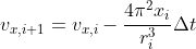
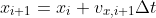
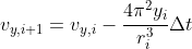
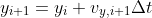
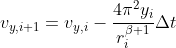
we next convert the equations of motion into difference equations in preparation for constructing a computational solution.We find
and I imitate it by python ,and I gained that:

code1触菜,as follows:
#coding:utf-8
import pylab as pl
import numpy as np
import math
from mpl_toolkits.mplot3d import Axes3D
import matplotlib.pyplot as plt
from matplotlib import animation

class circle():
    def __init__(self,x0=1,y0=0,t0=0,vx0=0,vy0=2*math.pi,dt0=0.001,total_time=10):
        self.x=[x0]
        self.y=[y0]
        self.vx=[vx0]
        self.vy=[vy0]
        self.R=x0**2+y0**2
        self.t=[t0]
        self.dt=dt0
        self.T=total_time
    def run(self):
        for i in range(int(self.T/self.dt)):
            vx=self.vx[-1]-(4*math.pi**2*self.x[-1]/self.R**2)*self.dt
            vy=self.vy[-1]-(4*math.pi**2*self.y[-1]/self.R**2)*self.dt
            self.vx.append(vx)
            self.vy.append(vy)
            self.x.append(self.vx[-1] * self.dt + self.x[-1])
            self.y.append(self.vy[-1] * self.dt + self.y[-1])
    def show(self):
        pl.plot(self.x, self.y, '-', label='tra')
        pl.xlabel('x(AU)')
        pl.ylabel('y(AU)')
        pl.title('Earth orbiting the Sun')
        pl.xlim(-1.2,1.2)
        pl.ylim(-1.2,1.2)
        pl.axis('equal')
        pl.show()
a=circle()
a.run()
a.show()
we can use the animation of matplotlib to gain the cartoon,
add follow codes:
 def drawtrajectory(self):
        fig=plt.figure()
        ax = plt.axes(title=('Earth orbiting the Sun'),
                      aspect='equal', autoscale_on=False,
                      xlim=(-1.1, 1.1), ylim=(-1.1, 1.1),
                      xlabel=('x'),ylabel=('y'))
        line=ax.plot([],[],'b')
        point=ax.plot([],[],'ro',markersize=10)
        images=[]
        def init():
            line=ax.plot([],[],'b',markersize=8)
            point=ax.plot([],[],'ro',markersize=10)
            return line,point
        def anmi(i):
            ax.clear()
            line=ax.plot(self.x[0:10*i],self.y[0:10*i],'b',markersize=8)
            point=ax.plot(self.x[10*i-1:10*i],self.y[10*i-1:10*i],'ro',markersize=10)
            return line,point
        anmi=animation.FuncAnimation(fig,anmi,init_func=init,frames=10000,interval=1,
                                     blit=False,repeat=False)
we get follow gif

If we consider the reduced mass
The orbital trajectory for a body of reduced mass is given in polar coordinates by
+\frac{1}{r}=-\frac{\mu r2}{L2} F(r))
consider
we have
\frac{1}{1-e cos\theta })
so
Then let us suppose that the gravitational force is of the form
then I get


the picture


code
#coding:utf-8
import pylab as pl
import numpy as np
import math
from mpl_toolkits.mplot3d import Axes3D
import matplotlib.pyplot as plt
from matplotlib import animation

class circle():
    def __init__(self,x0=1,y0=0,t0=0,vx0=0,vy0=1.7*math.pi,dt0=0.001,Beta=2.3,total_time=10):
        self.x=[x0]
        self.y=[y0]
        self.vx=[vx0]
        self.vy=[vy0]
        self.t=[t0]
        self.dt=dt0
        self.T=total_time
        self.beta=Beta
    def run(self):
        for i in range(int(self.T/self.dt)):
            R=(self.x[-1]**2+self.y[-1]**2)**0.5
            vx=self.vx[-1]-(4*math.pi**2*self.x[-1]/R**(self.beta+1))*self.dt
            vy=self.vy[-1]-(4*math.pi**2*self.y[-1]/R**(self.beta+1))*self.dt
            self.vx.append(vx)
            self.vy.append(vy)
            self.x.append(self.vx[-1] * self.dt + self.x[-1])
            self.y.append(self.vy[-1] * self.dt + self.y[-1])
    def show(self):
        pl.plot(self.x, self.y, '-', label='tra')
        pl.xlabel('x(AU)')
        pl.ylabel('y(AU)')
        pl.title('Earth orbiting the Sun')
        pl.xlim(-1,1)
        pl.ylim(-1,1)
        pl.axis('equal')
        pl.show()
    def drawtrajectory(self):
        fig=plt.figure()
        ax = plt.axes(title=('Earth orbiting the Sun '),
                      aspect='equal', autoscale_on=False,
                      xlim=(-1.1, 1.1), ylim=(-1.1, 1.1),
                      xlabel=('x'),ylabel=('y'))
        line=ax.plot([],[],'b')
        point=ax.plot([],[],'ro',markersize=10)
        images=[]
        def init():
            line=ax.plot([],[],'b',markersize=8)
            point=ax.plot([],[],'ro',markersize=10)
            return line,point
        def anmi(i):
            ax.clear()
            line=ax.plot(self.x[0:10*i],self.y[0:10*i],'b',markersize=8)
            point=ax.plot(self.x[10*i-1:10*i],self.y[10*i-1:10*i],'ro',markersize=10)
            return line,point
        anmi=animation.FuncAnimation(fig,anmi,init_func=init,frames=100000,interval=1,
                                     blit=False,repeat=False)
        plt.show()


a=circle()
a.run()
a.show()
#a.drawtrajectory()
then we get the animation

for the problem 4.8, I use the follow code to calculate
import pylab as pl
import numpy as np
import math
class circle():
    def __init__(self,x0=0.72,y0=0,t0=0,vx0=0,dt0=0.001,Beta=2.0,total_time=10,e0=0.007):
        self.x=[x0]
        self.y=[y0]
        self.vx=[vx0]
        self.vy=[]
        self.t=[t0]
        self.dt=dt0
        self.T=total_time
        self.beta=Beta
        self.e=e0

    def run(self):
        vy0=2*math.pi*(1-self.e)/math.sqrt(1+self.e)
        self.vy.append(vy0)
        for i in range(int(self.T/self.dt)):
            R=(self.x[-1]**2+self.y[-1]**2)**0.5
            vx=self.vx[-1]-(4*math.pi**2*self.x[-1]/R**(self.beta+1))*self.dt
            vy=self.vy[-1]-(4*math.pi**2*self.y[-1]/R**(self.beta+1))*self.dt
            self.vx.append(vx)
            self.vy.append(vy)
            self.x.append(self.vx[-1] * self.dt + self.x[-1])
            self.y.append(self.vy[-1] * self.dt + self.y[-1])
            self.t.append(self.t[-1]+self.dt)
            if(self.y[-1]<0):
                a=(self.x[0]-self.x[-1])/2
                T=2*self.t[-1]
                k=T**2/a**3
                break
        print(k)
a=circle()
a.run()
