Transformations
Your goal during the data gathering phase is to record as much working data about your observations as possible since you never know which feature is going to end up being the golden one that allows your machine learning algorithm to succeed. Due to this, there are usually a few redundant or even poor features in your dataset. Think back to those long word problems in grade school that were essentially a simple math question, but came filled with red herrings to throw you off; feeding an unfiltered soup of features to your machine learning algorithms is pretty similar to trying to get it to solve those word problems.
To be effective, many machine learning algorithms need the data passed to them be discerning, discriminating and independent. In this module, you're going to discover methods to get your data behaving like that using transformers. This will help improve your own knowledge of your data, as well as improve your machine learning algorithms' performance.
A transformer is any algorithm you apply to your dataset that changes either the feature count or feature values, but does not alter the number of observations. You can use transformers to mung your data as a pre-processing step to clean it up before it's fed to other algorithms. Another popular transformer use is that of dimensionality reduction, where the number of features in your dataset is intelligently reduced to a subset of the original.
Once you've used a few basic transformers, you will also learn about some data cleansing techniques that attempt to rectify problematic observations.
PCA
Unsupervised learning aims to discover some type of hidden structure within your data. Without a label or correct answer to test against, there is no metric for evaluating unsupervised learning algorithms. Principal Component Analysis (PCA), a transformation that attempts to convert your possibly correlated features into a set of linearly uncorrelated ones, is the first unsupervised learning algorithm you'll study.
What is principal component analysis?
PCA falls into the group of dimensionality reduction algorithms. In many real-world datasets and the problems they represent, you aren't aware of what specifically needs to be measured to succinctly address the issue driving your data collection. So instead, you simply record any feature you can derive, usually resulting in a higher dimensionality than what is truly needed. This is undesirable, but it's the only reliable way you know to insure you capture the relationship modeled in your data.
If you have reason to believe your question has a simple answer, or that the features you've collected are actually many indirect observations of some inherent source you either cannot or do not know how to measure, then dimensionality reduction applies to your needs.
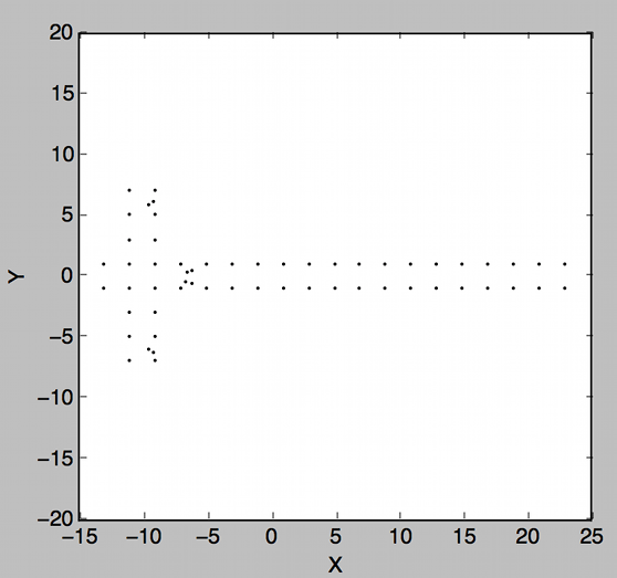
PCA's approach to dimensionality reduction is to derive a set of degrees of freedom that can then be used to reproduce most of the variability of your data. Picture one of those cartoon style telephone poles; once you have a figure in mind, compare it to this one:

Your envisioned image probably looked similar. You could have pictured it from any other viewing angle, for instance, as if you were floating directly above it looking down:

However you probably didn't, since that view doesn't contain enough variance, or information to easily be discernible as a telephone pole. The frontal view, however, does. Looking at a telephone pole or any other object from various viewing angles gives you more information about that object. If the view angles are really close to one another, the information you get from the views ends up being mostly the same, with a lot of duplicate information. However if you're able to move to a completely different angle, you can get a lot more information about the object you're examining. And if you're wisein choose your view angles, with just a few calculated glimpses of an object, you can build a rather comprehensive understanding of it. PCA calculates those best view angles:

How Does PCA Work?
PCA is one of the most popular techniques for dimensionality reduction, and we recommend you always start with it when you have a complex dataset. It models a linear subspace of your data by capturing its greatest variability. Stated differently, it accesses your dataset's covariance structure directly using matrix calculations and eigenvectors to compute the best unique features that describe your samples.
An iterative approach to this would first find the center of your data, based off its numeric features. Next, it would search for the direction that has the most variance or widest spread of values. That direction is the principal component vector, so it is then added to a list. By searching for more directions of maximal variance that are orthogonal to all previously computed vectors, more principal component can then be added to the list. This set of vectors form a new feature space that you can represent your samples with.
On Dimensions, Features, and Views
Each sample in your dataset represents an observable phenomenon, such as an object in the real world. Each feature in your dataset tells you details about your samples. Recall from earlier chapters that features and views are synonymous terms; this isn't accidental! Just like looking at an object from different views gives you more information about the object, so too does examining a sample from different features. Similar or correlated features will produce an "overlapped" view of your samples, the same way similar views of an object also overlap.
PCA ensures that each newly computed view (feature) is orthogonal or linearly independent to all previously computed ones, minimizing these overlaps. PCA also orders the features by importance, assuming that the more variance expressed in a feature, the more important it is. In our telephone pole example, the frontal view had more variance than the bird's-eye view and so it was preferred by PCA.
With the newly computed features ordered by importance, dropping the least important features on the list intelligently reduces the number of dimensions needed to represent your dataset, with minimal loss of information. This has many practical uses, including boiling off high dimensionality observations to just a few key dimensions for visualization purposes, being used as a noise removal mechanism, and as a pre-processing step before sending your data through to other more processor-intensive algorithms. We'll look at more real life use cases in the next unit.
When Should I Use PCA?
PCA, and in fact all dimensionality reduction methods, have three main uses:
To handle the clear goal of reducing the dimensionality and thus complexity of your dataset.
To pre-process your data in preparation for other supervised learning tasks, such as regression and classification.
To make visualizing your data easier, since we can only perceive three dimensions simultaneously.
According to Nielson Tetrad Demographics, the group of people who watch the most movies are people between the ages of 24 through 35. Let's say you had a list of 100 movies and surveyed 5000 people from within this demographic, asking them to rate all the movies they've seen on a scale of 1-10. By having considerably more data samples (5000 people) than features (100 ordinal movie ratings), you're more likely to avoid the curse of dimensionality.
Having collected all that data, even though you asked 100 questions, what do you think truly is being measured by the survey? Overall, it is the collective movie preference per person. You could attempt to solve for this manually in a supervised way, by break down movies into well-known genres:
Action
Adventure
Comedy
Crime & Gangster
Drama
Historical
Horror
Musicals
Science Fiction
War
Western
etc.
Being unsupervised, PCA doesn't have access to these genre labels. In fact, it doesn't have or care for any labels whatsoever. This is important because it's entirely possible there wasn't a single western movie in your list of 1000 films, so it would be inappropriate and strange for PCA to derive a 'Western' principal component feature. By using PCA, rather than you creating categories manually, it discovers the natural categories that exist in your data. It can find as many of them as you tell it to, so long as that number is less than the original number of features you provided, and as long as you have enough samples to support it. The groups it finds are the principal components, and they are the best possible, linearly independent combination of features that you can use to describe your data.
One warning is that again, being unsupervised, PCA can't tell you exactly what the newly created components or features mean. If you're interested in how to interpret your principal components, we've included two sources in the dive deeper section to help out with that and highly recommend you explore them.
Once you've reduced your dataset's dimensionality using PCA to best describe its variance and linear structure, you can then transform your movie questionnaire dataset from its original [1000, 100] feature-space into the much more comfortable, principal component space, such as [1000, 10]. You can visualize your samples in this new space using an Andrew's plot, or scatter plot. And finally, you can base the rest of your analysis on your transformed features, rather than the original 100 feature dataset.
PCA is a very fast algorithm and helps you vaporizes redundant features, so when you have a high dimensionality dataset, start by running PCA on it and then visualizing it. This will better help you understand your data before continuing.
Projecting a Shadow
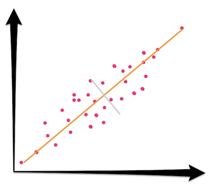
By transforming your samples into the feature space created by discarding under-prioritized features, a lower dimensional representation of your data, also known as shadow or projection is formed. In the shadow, some information has been lost—it has fewer features after all. You can actually visualize how much information has been lost by taking each sample and moving it to the nearest spot on the projection feature space. In the following 2D dataset, the orange line represents the principal component direction, and the gray line represents the second principal component. The one that's going to get dropped:

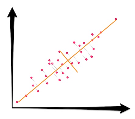
By dropping the gray component above, the goal is to project the 2D points onto 1D space. Move the original 2D samples to their closest spot on the line:

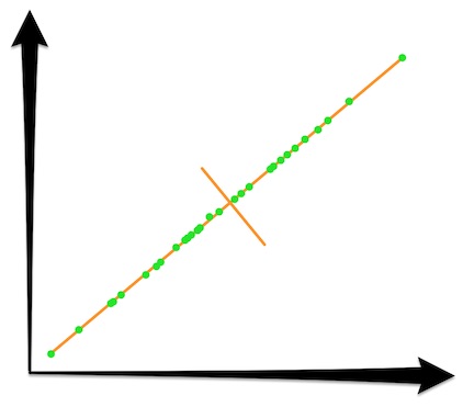
Once you've projected all samples to their closest spot on the major principal component, a shadow, or lower dimensional representation has been formed:

The summed distances traveled by all moved samples is equal to the total information lost by the projection. An an ideal situation, this lost information should be dominated by highly redundant features and random noise.